Quantcast
Channel: QGIS Planet
Viewing all 1090 articles
Browse latest View live

QGIS UK: 8th Scottish QGIS UK user group meeting plans

$
0
0

It’s been a long time since we posted anything up here but hopefully the news of another user group happening in Stirling on 7th November will hopefully assuage your distress.

The event is very kindly hosted by Historic Environment Scotland in their restored Engine Shed and is also supported by Ordnance Survey, Cawdor Forestry, thinkWhere, SEPA and Registers of Scotland.

The programme is still being worked out but plan on attending one of two workshop sessions in the morning run by Ordnance Survey and thinkWhere and then a full afternoon of presentations and lightning talks.

Tickets are available through Eventbrite.

8th Scottish QGIS @UK user group


QGIS NL Community: Dutch QGIS usergroup meeting

$
0
0
All presentations will be in Dutch. Please have a look at the Dutch version of this page to see more…

North Road: Edit Features “In Place” crowdfund — made it to QGIS 3.4!

$
0
0

Well, thanks to the resounding success of our QGIS edit-in-place crowdfunding campaign, we’ve been frantically smashing away at our keyboards in an attempt to reward the QGIS community by sneaking this feature in a whole 4 months earlier than originally promised! And, we’re very proud to announce, that this exciting new feature has been implemented and will be included in the upcoming QGIS 3.4 release (due late October 2018). So go ahead — grab one of the nightly pre-release of QGIS 3.4 and checkout the results.

This wouldn’t have been possible without the rapid response to the campaign and the generosity of our wonderful backers:

(In addition to these backers, we’ve also received numerous anonymous donations to this feature from many other individuals — while we can’t list you all publicly, you’re also in our thanks!)


Keep an eye on this blog for other upcoming QGIS crowdfunding campaigns targeted at QGIS 3.6 and beyond… we’ve got lots more exciting work planned for these releases!


QGIS NL Community: Programme change…

$
0
0
See the Dutch website for more info on the programme.

Ireland QGIS User Group Blog: Add Realistic Mist and Fog to Topography in QGIS 3.2

$
0
0

I recently came across a great tutorial by in which he demonstrated how to create map of Switzerland in the style of Edward Imhof, the famed Swiss cartographer renowned for his hand painted maps of Switzerland and other mountainous regions of the world. John’s map used traditional hillshading, multidirectional hillshading and crucially, a translucent topographic layer that created a mist like appearance he likened to the sfumato technique used by painters since the Renascence.

I followed John’s tutorial in QGIS 3.2 and I was quite pleased with the initial result below. However, the process creating it is a bit too complicated for a tutorial so I set about simplifying the process and rather than imitating Imhof’s distinct style, my goal this time is realism.

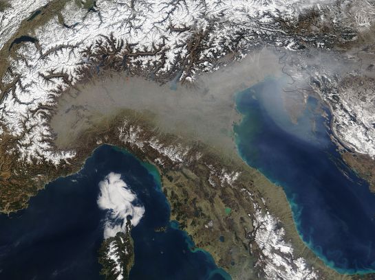
The heart of the effect involves the very clever idea of using the topographic layer as a subtle opacity mask to simulate mist, fog and atmospheric haze. Have a look at the image below taken on March 17th, 2005 by NASA’s Terra satellite. This is the industrialised Po valley of northern Italy, surrounded by the Alps and Apennine Mountains that rise above the valley’s hazy pollution. The haze adds a sense of depth to the surrounding hills and mountains. It’s not uncommon to see fog and pollution in satellite imagery that gives way to the clear air in high mountains e.g. northern India and Nepal, China, Pakistan and India. Creating a similar mist effect in QGIS is actually quite simple.

First download topography for the Alps and Po region (a 68.55 Mb GeoTiff file derived from freely available EU-DEM data I resampled from 25 to 100m resolution). Next, make sure you have the plugin QuickMapServics (QMS) installed (menu Plugins – Manage and Install Plugins). This great plugin provides access to over 1000 basemaps.

Load the GeoTiff file into QGIS (Raster – Load) and rename the layer Hillshade. Right click the layer to open the Layer Properties window. In the Symbology panel, next to Render Type, choose Hillshade. Change the altitude to 35 degrees, Azimuth to 300 degrees and Z Factor of 1.5 (illuminating the landscape from the top left). Finally, change the Blending mode to Multiply. Click OK to close the dialogue.

To add the basemap layer, Esri World Imagery (Clarity), type “ESRI clarity” in the QMS search bar to find and add the basemap; Go to View – Panels and activate the QMS search bar if it isn’t initially visible. Make sure it’s the bottommost layer.

Oh, that’s a bit disappointing, we only increased the relief little a bit. It’s missing the vitally important mist layer.

To create mist, right click the Hillshade layer and choose Duplicate. Rename the new layer Mist and make sure it’s above the Hillshade layer. Now open the Layer Properties window of the layer, we’re going edit it’s attributes to make it look like mist.

Change the Render type to Singleband Pseudocolor and use 0 and 3000 for the min and max values (limiting maximum latitude of the mist to 3000 meters). Then open the colour ramp window by clicking on the Color ramp and enter these values:

  • Left Gradient – HSV 215 15 50 and 75% transparency
  • Right Gradient – HSV 215 15 50 and 0% transparency

Close the Color Ramp dialogue. In the Layer Properties window, and this is very important, change the Blending mode to Lighten. Click OK to close the Layer Properties window.

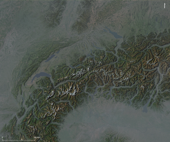
Wow, we have mist!

The mist effect looks great. It certainly adds a lot of realism to the topographic map, it now looks quite like NASA’s images. This is just a quick and basic map so there’s lots of scope to improve the effect. Play around with the colour of the mist layer and its opacity, or even brighten the Hillshade layer underneath. See what effects these changes have.

Here’s another example below. In this example I duplicated the hillshade layer and set the second hillshade layer to Multidirectional Hillshading (yes, QGIS 3.2 has Multidirectional Hillshading). I then adjusted the transparency of both hillshade layers so they blended together nicely. I then replaced the basemap with another duplicated topography layer that I coloured using the gradient sd-a (by Jim Mossman, 2005) using the cpt-city plugin. And lastly, I doubled the opacity of the mist layer turning it into a milky fog. I think it looks great!

What next? Well, there’s lots of possibilities. Perhaps download Martian topography and add mist to the bottom of Valles Marineris?

References:

Eduard Imhof – Biography

TV documentary about Eduard Imhof

The Map as an Artistic Territory: Relief Shading Works and Studies by Eduard Imhof

Haze in northern Italy – NASA Terra Satellite

Tzvetkov, J., 2018. Relief visualization techniques using free and open source GIS tools. Polish Cartographical Review, 50(2), pp.61-71.

Lutra Consulting: New 3D features in QGIS 3.4

$
0
0

Thanks to the great response from the QGIS community to our crowdfunding call, we have added several new features to the upcoming release (3.4).

Here are the highlights of the features:

Print layout

With this new feature, you can embed a 3D scene to the print layout. In addition, there are camera and view setting tools available to adjust the scene from within the map frame. This will allow you to generate high resolution outputs similar to the other map frames.

QGIS 3D configuration

Animation

You can create an animation based on a set of keyframes - camera positions at particular times. QGIS 3D then interpolates the camera positions/rotations in between the keyframes.

To create the keyframes, first set the scene for your map, by rotating, zooming or moving the camera. Then assign a time to the frame. There are several methods for interpolations between keyframes.

QGIS 3D configuration

3D lines

If you have a 3D linestring, you can now use the elevation of vertices to display it in 3D map.

QGIS 3D configuration

Camera control

There are more control on how you can pan, rotate and zoom the camera within the scene:

  • Page up/down: to move the camera up/down: Page up/down keys for moving the camera
  • Free camera movements: also possible to look from below: Page up/down keys for moving the camera
  • Shift key and drag: the camera rotates around a point on terrain: Page up/down keys for moving the camera
  • Ctrl key and drag: this will rotate camera while it stays in one position Page up/down keys for moving the camera

In addition, the point towards which the camera is looking is dynamically adjusted based on the terrain. The rotation in scenes where a DEM used for terrain has been enhanced significantly. This is more pronounced with presence of higher hills in the terrain.

Further development

There are still some exciting features from the crowdfunding which will be incorporated in QGIS 3.6. You can check the QGIS development or follow us on Twitter.

Lutra Consulting: Mesh Data Abstraction Library (MDAL)

$
0
0

In the world of GIS, vector and raster are the most common data types to represent real world features. But not always, vectors and rasters can describe the complexity and nature of the data.

MDAL Mesh

Example of those datasets are:

  • Metrological data: e.g. temperature and wind speed
  • Hydrological data: flood depth and flow velocity
  • Oceanography: salinity and wave flux

MDAL arrows and contours

In the past, we introduced Crayfish plugin to handle unstructured grids, usually with temporal and other components. The main issues with Crayfish plugin were:

  • Crayfish plugin had its own renderer. Therefore, we had to create binaries and ship them with the plugin. This was not ideal, as not all the platforms (e.g. MacOS) was not supported.
  • Crayfish plugin loaded all the data in the memory. For small files, this was not an issue. But there was not a solution for larger files.

Why MDAL?

For more details of the rational behind introducing MDAL, see the QGIS Enhancement Proposal with great suggestions and feedback from the developers.

TL;DR: we needed a new abstraction library to handle the mesh data formats similar to GDAL/OGR dealing with rasters and vectors.

Current state

After the feedback from the QGIS community, we have introduced MDAL library earlier this year. It took us a bit of time to put the infrastructure in place. There are already some formats available from MDAL. The library was integrated to QGIS from 3.2. But extensive improvements and new features were added during 3.4.

There are still more formats to support. In QGIS, we will also need to enhance the spatial indexing and performance of the driver in general. For more information visit MDAL website.

How to work with MDAL layer in QGIS

Here is a mesh layer you can use to load in QGIS. For more data, you can visit the ECMWF(or Copernicus) or NASA websites.

In QGIS, from the main menu > Layer > Data Source Manager. A new window will appear. From the left panel, click on Mesh layerMesh and point to the downloaded file.

You should be able to see a figure similar to the one below:

Mesh layer in QGIS

To view quantities within the mesh, you can open the Layer Styling Panel. Click on symbology Styling tab:

  • First select symbology and deactivate Native Mesh Rendering
  • Click on general and under groups, towards the right of 10 metre wind click on contour and vector to view the quantities.
  • Below the Groups, you can move the slider to browse through time of the dateset(s).
  • To change style of the contours and vectors you can click on contour and vector tabs and adjust the color ramps and vector sizes accordingly.

Mesh layer in QGIS

What happens to Crayfish plugin?

We have recently released a new version of Crayfish plugin to work directly with mesh layer in QGIS. Crayfish is now based on Python only and can be installed on all main platforms (including MacOS).

Future developments

We are planning to add mesh calculator (either as a core QGIS feature or Crayfish/Processing plugin). There will be more formats in the pipeline to support in MDAL too.

If you’d like to add support for your mesh layer to MDAL, you can follow the examples on the github repository. We are always happy to help.

QGIS Project blog: QGIS 3.4 Madeira is released!

$
0
0

We are pleased to announce the release of QGIS 3.4 ‘Madeira’! Madeira was the location of our developer meeting in February 2018.

Windows installers and Ubuntu/debian binaries are already out, and all the packagers are actively preparing packages for the other operating systems. We’ll keep you updated when different packages and installers become available.

QGIS 3.4 will become the first LTR of version 3. Based on our current plans, 3.4 will replace 2.18 as LTR in February 2019.

We would like to thank the developers, documenters, testers and all the many folks out there who volunteer their time and effort (or fund people to do so). From the QGIS community we hope you enjoy this release! If you wish to donate time, money or otherwise get involved in making QGIS more awesome, please wander along to qgis.org and lend a hand!

QGIS is supported by donors and sponsors. A current list of donors who have made financial contributions large and small to the project can be seen on our donors list. If you would like to become and official project sponsor, please visit our sponsorship page for details. Sponsoring QGIS helps us to fund our six monthly developer meetings, maintain project infrastructure and fund bug fixing efforts. A complete list of current sponsors is provided below – our very great thank you to all of our sponsors!

QGIS is Free software and you are under no obligation to pay anything to use it – in fact we want to encourage people far and wide to use it regardless of what your financial or social status is – we believe empowering people with spatial decision making tools will result in a better society for all of humanity.


Markus Neteler: GRASS GIS 7.4.2 released

$
0
0

We are pleased to announce the GRASS GIS 7.4.2 release

What’s new in a nutshell

After a bit more than four months of development the new update release GRASS GIS 7.4.2 is available. It provides more than 50 stability fixes and improvements compared to the previous stable version 7.4.1. An overview of the new features in the 7.4 release series is available at New Features in GRASS GIS 7.4.

Efforts have concentrated on making the user experience even better, providing many small, but useful additional functionalities to modules and further improving the graphical user interface. Segmentation now support extremely large raster maps. Dockerfile and Windows support received updates. Also the manual was improved. For a detailed overview, see the list of new features. As a stable release series, 7.4.x enjoys long-term support.

Binaries/Installer download:

Source code download:

More details:

See also our detailed announcement:

About GRASS GIS

The Geographic Resources Analysis Support System (https://grass.osgeo.org/), commonly referred to as GRASS GIS, is an Open Source Geographic Information System providing powerful raster, vector and geospatial processing capabilities in a single integrated software suite. GRASS GIS includes tools for spatial modeling, visualization of raster and vector data, management and analysis of geospatial data, and the processing of satellite and aerial imagery. It also provides the capability to produce sophisticated presentation graphics and hardcopy maps. GRASS GIS has been translated into about twenty languages and supports a huge array of data formats. It can be used either as a stand-alone application or as backend for other software packages such as QGIS and R geostatistics. It is distributed freely under the terms of the GNU General Public License (GPL). GRASS GIS is a founding member of the Open Source Geospatial Foundation (OSGeo).

The GRASS Development Team, October 2018

The post GRASS GIS 7.4.2 released appeared first on GFOSS Blog | GRASS GIS and OSGeo News.

QGIS Project blog: Report back on the 20th QGIS Hackfest in Zanzibar

$
0
0


This post summarizes personal reports of community members who attended the 20th Hackfest in Stone Town, Zanzibar the week before the FOSS4G in Dar Es Salaam.

Report from Matteo Ghetta

QGIS developers spent 3 days in the beautiful island of Zanzibar were they worked on bug fixing, improvement of new features and documentation enhancements. It is extremely important for developers to meet together and spend some days working side by side given that the geographical distribution is very wide.

Thanks to the (local government & Yves Barthelemy) we had the chance to visit the Land Mapping Commission in Stone Town: It has been an amazing experience for both developers and local council. Moreover developers visited the SUZA (University of Zanzibar) and saw the local infrastructure and GIS related workflow.

  • I have merged many PR of the documentation
  • Many old and not old issues have been closed or the author has been pinged
  • Many new additions to the documentation both small corrections and new sections from scratch
  • A new version of DataPlotly released
  • A small presentation of DataPlotly to the QGIS crew

Report from Mario Baranzini

I spent one day of the Hackfest contributing to the SLYR project, improving the conversion of LAB colors. SLYR (https://github.com/nyalldawson/slyr) is a project started and almost entirely developed by Nyall (which was not present to the Hackfest) which aims to provide tools to extract and convert symbols from ESRI .lyr and .style files and use them in QGIS. Nyall has recently worked hard on the project and perhaps soon sponsorship will allow further development.

Around this theme there is a keen interest. Even during the FOSS4G there has been discussion of the conversion of ESRI symbols and there was also a presentation of how the conversion in Israel is currently managed.

During the rest of the hackfest, I worked on the implementation of the new QField file selector.

Report from Denis Rouzaud

Report from Tim Sutton

Firstly let me thank the QGIS project for contributing to my travel and accommodation costs – I am most grateful for the support! This hackfest was special for me because it is the first hackfest in an African country. As an African born person living in the interface between “first world” and “third world”, I have always had a particular social agenda with QGIS: To bring spatial tools to support responsible and sustainable management of our world. There is a huge technological and skills divide between Europe and less developed societies where QGIS can be a valuable social enabler in helping to advance the standard of living and quality of life. Hosting a hackfest in an environment where we don’t have tree cadastres, street furniture cadastres and every aspect of civilian life mapped and systematised is an important way to build empathy and understanding in our QGIS core community members for a broader cross-section of our user base. Having the opportunity to meet with users from ZMI (the Zanzibar Mapping Initiative) and students from the local university was a really uplifting experience. ZMI are building the national cadastre from the ground up using QGIS, PostGIS and UAV mapping. We were privileged to have a number of Zanzibar residents join us on the hackfest and get to experience just how appreciative they are, first hand.

There were a number of interesting topics that arose during the hackfest which I will try to summarise here:

Certification:

We held an extended meeting on the QGIS Certification Programme, mainly detailing how we should go about the review process for onboarding new organisations.

Mac OS Build:

I spent quite a bit of time struggling with my MacOS build on QGIS. It’s definitely an area of the project that needs more work as the process can be non-trivial and the brew based formulas quickly become outdated.

QField Show and Tell:

Matthias showed off the latest version of QField and all the hard work they have been putting into the QGIS mobile client. This Android based version of QGIS for mobile data gathering is a really great project and is getting more and more useful with each release. There was also a translation sprint for QField during which I translated it to Afrikaans.

QField Autobuilds:

Denis and Matthias showed off the work they have done to automate the .apk builds for QField. Their system combines Travis and some git hooks to automatically build .APK’s whenever a pull request os made or a tag is made. See the QField travis for details: https://github.com/opengisch/QField/blob/master/.travis.yml

Plotly plugin:

Matteo Ghetta showed off the latest capabilities of the Data Plotly plugin for QGIS 3. The plugin supports the creation of a wide assortment of charts from your layer’s attribute data. See the plugin homepage here for examples and more detail: https://github.com/ghtmtt/DataPlotly 

Governance:

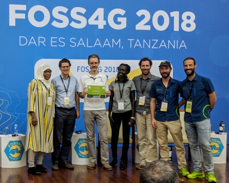
I took the opportunity to sign off the statute changes from 2017 general meeting. This was my last official act as outgoing project Chair. I was also extremely humbled to be awarded an Honorary PSC membership during the FOSS4G2018 conference.

TimRecievesHonoraryPSCMembership
Easter Eggs:

I contributed a couple of new easter eggs to QGIS. While easter eggs are fun, the data behind these hidden tools provide an important history of the project. I took the opportunity of having many long-time QGIS community members around the dinner table to collate all the previous QGIS meet-up dates. You can view this as a map here: https://github.com/qgis/QGIS/blob/master/resources/data/qgis-hackfests.json 

The spatial clustering of these events shows that going to Zanzibar and getting out of our geographical comfort zone is a really useful endeavour.

Report from Paolo Cavallini

During the HF in Zanzibar I mainly worked on:

  • Plugins: I cleaned up the queue of unapproved plugins, contacting all individual authors, fixing what was possible and deprecating the worst cases; we also solved a long standing issue with a contentious plugin
  • Issues: I examined many tickets, especially those waiting for feedback
  • Training certification: through a very productive meeting we defined clear rules for accepting certifying organizations, with the main aim of driving people to actively support the project:
    • in the application process, the proponent should explain what are his contribution to QGIS project
    • following an initial review, the application will be sent to local QGIS groups for their opinion, which should take place in less than one monthly; where there is no user group, the responsibility will fall entirely on PSC shoulders
    • the training material for each course should be released with a free license, and a review will be done; if the material is not of adequate quality, this is a cause for refusal
    • then PSC will take a decision and publish the contributions as stated by the proponent, for transparency
  • Other meetings helped focusing on our mission, defining the relationship between volunteer and paid work, and other
  • I visited the Land Mapping Commission and the University, soliciting a tighter cooperation with QGIS project.

Report from Admire Nyakudya

During the heck fest in Zanzibar, I mainly worked on porting some common plugin we use to QGIS 3. The plugins I mainly worked on were Cogo Parcel plugin and Sg Diagram downloader. We visited the Zanzibar mapping agency and interacted with the people who were working on capturing cadastral data using QGIS and explained them about the COGO Parcel plugin which streamlines capturing cadastral boundaries in QGIS and storing the results in a PostgreSQL database. To summarise the work I was working on during the heck fest.

  • Port Cogo Plugin from QGIS 2 to make it compatible with QGIS 3. This has been achieved and now awaiting one of my team members to approve the pull request.
  • Expand functionality being offered by the COGO Parcel plugin to include the new reporting framework in QGIS 3.
  • Investigate ways to generate projects on the fly after talking to Matteo and seeing the work he has done with QGIS project generator.

I also went to the Zanzibar university to see ways in which QGIS is being used in the local university and how students are integrating drone imagery with QGIS.

Report from Matthias Kuhn

The highest value of hackfests is actually to meet and greet and discuss ideas and bigger plans. There is a lot of communication on a high bandwidth channel (also known as face-to-face) that strengthens the community. This helps to quickly overcome technical problems sometimes. Or to give someone some tips and tricks you normally wouldn’t come to (e.g. optimizing a git workflow) that results in a long-term gain because of sustainable productivity improvements. I tend to walk around once in a while and just randomly bump into people where I – more or less successfully – try to help them solve their issues or discuss approaches. In the same area, there is the possibility to informally discuss plans about organization, workflows and strategies. The concept of an LTR was to a big degree discussed and built at a hackfest in Essen some years ago. This year there was a very interesting discussion about the topic LTR. For how much time the “long” in the term “long term release” should stand, about the life cycle of releases and of long-term releases. One of the important things when it comes to this question is what organisations think and do – because, in the end, it is mostly for organisations that the LTR exists – and how development resources can be assigned to the task of keeping a high quality of an LTR during its whole lifetime. There are no conclusions yet, but synchronizing on these ideas is often the seed for tomorrow’s exciting changes.

We were also visited by a group of students from the local university. It was really refreshing to talk to them about open source and QGIS and how we work and what the challenges of spatial data and GIS infrastructure are on an island like Zanzibar.

Feature-wise, the main thing I worked on feature wise was a new snap to grid functionality that is available for digitizing tools. It allows configuring a precision for vector layers. Whenever a new node is added or an existing one is edited on this vector layer, it will be automatically placed on this grid. Normally this is used to force the objects on a layer to something like cm or mm resolution.

And then, of course, I did my daily bunch of (mostly volunteer) pull request reviewing, some code cleanup and some bugfixes.

Report from Marco Bernasocchi

https://photos.app.goo.gl/seX2kSJ9vKxKBZt58

The Zanzibar hackfest was a special one for me, my first hackfest as QGIS.org co-chair. My main goal was definitely to get as much information out of Tim as possible so that I wouldn’t have to keep on bugging him all time 🙂

Beside that, multiple meetings where planned to which I took part, as Paolo already explained, we had very good meetings about:

  • Certifications meeting
  • Trademark discussion
  • Creating a membership system that allows entities that are not allowed to budget sponsoring money to instead become paying members.
  • Other meetings helped focusing on our mission, defining the relationship between volunteer and paid work, and other

On the first two days, we were joined by a largish group of local students to whom I explained how the structure of QGIS.org works and where they could help. I also helped them choosing a task to work and mentored them.

As I mentioned before, I spent a lot of time asking a lot of questions to Tim to get the biggest possible knowledge transfer about running QGIS.org and some time choosing and booking restaurants for our evening “meetings”

On the technical side, I worked with Mario on a new implementation of the QField File selector.

After everybody left, the OPENGIS.ch team stayed one day longer and introduced Mario to the real Brighton-style hackfest with take-away pizza 😉


ANDROID · GIS · WEB: The new QML widgets in QGIS – When widgets get unbridled

$
0
0
Individuality is the definition of freedom. And freedom is the fundamental requirement of man’s mind. QGIS possibly cannot give you all the freedom you require in life. But at least a lot of freedom in how you manage your work.
See more ›

QGIS NL Community: (Nederlands) BGT Import plugin vernieuwd

$
0
0
Sorry, this entry is only available in the Dutch language

anitagraser.com: My favorite new recipe in QGIS Map Design 2nd ed

$
0
0

If you follow me on Twitter, you have probably already heard that the ebook of “QGIS Map Design 2nd Edition” has now been published and we are expecting the print version to be up for sale later this month. Gretchen Peterson and I – together with our editor Gary Sherman (yes, that Gary Sherman!) – have been working hard to provide you with tons of new and improved map design workflows and many many completely new maps. By Gretchen’s count, this edition contains 23 new maps, so it’s very hard to pick a favorite!

Like the 1st edition, we provide increasingly advanced recipes in three chapters, each focusing on either layer styling, labeling, or creating print layouts. If I had to pick a favorite, I’d have to go with “Mastering Rotated Maps”, one of the advanced recipes in the print layouts chapter. It looks deceptively simple but it combines a variety of great QGIS features and clever ideas to design a map that provides information on multiple levels of detail. Besides the name inspiring rotated map items, this design combines

  • map overviews
  • map themes
  • graduated lines and polygons
  • a rotated north arrow
  • fancy leader lines

all in one:

“QGIS Map Design 2nd Edition” provides how-to instructions, as well as data and project files for each recipe. So you can jump right into it and work with the provided materials or apply the techniques to your own data.

The ebook is available at LocatePress.

QGIS Project blog: User question of the Month – Nov 18

$
0
0

QGIS 2.18 is the third LTR since we started this effort back in 2015 and next year will see the first LTR of QGIS 3. On this occasion, we want to learn more about our users and which versions of QGIS they use. Therefore, we invite you to our QGIS user question of the month.

ANDROID · GIS · WEB: Visualize Postgres JSON data in QML widgets

$
0
0
As promised some time ago in “The new QML widgets in QGIS – When widgets get unbridled” we still owe you some fancy unicorns, but first let’s have a look at another nice feature that has been introduced in QGIS 3.4
See more ›

ANDROID · GIS · WEB: QGIS speaks a lot of languages

$
0
0

QGIS is a real cosmopolitan. Born in Alaska sixteen years ago, it has spread all over the world since. Thanks to its open source mentality, it finds not only in economically strong countries big usergroups. No question, that beside all the developers, there is a bunch of brave translators giving everything to make and keep QGIS multilingual. It’s translated in over forty languages – even to Mandarin Chinese and Esperanto. Not only the application, but also its plugins.
And since the feature-loaded long term release 3.4.0 even the QGS-Projects themselves.  Thanks to the friendly support of QGIS Usergroup Switzerland and the QGEP Project.

How it comes

Plugins are often shipped with pre-configured project files. To provide them in the users individual language, you’ve been required to translate the project manually in the properties and store it separately. When you needed to change something, you have been coerced to update every single file. This is a big effort and fault-prone. So there appeared the idea to have translation files for each required language, and when the user opens the only one project, it will be translated to his specific language. And that’s, what this new functionality does.

How it’s done

Like QGIS and the plugins, the projects are translated with the Qt translation process. Means, it makes the translation according to a Qt Compiled Translation Source File (.qm file). When the user opens a project, QGIS checks for a .qm file laying in the same folder like the .qgs file, having the same name like the .qgs file and having the language-code as postfix of the users language (the language configured in the QGIS settings).
So when the user opens a project named “citybees.qgs” that is originally in English, but his QGIS language is German, it checks for a file named “citybees_de.qm”. The project’s layer names, field-aliases, container names and much more will be translated to German and the project will be automatically stored as “citybees_de.qgs”. So the user has his German project version and can use and edit it like he wishes. Super easy.

Start from the beginning

Swiss people love honey and so they are diligent beekeepers. So, let’s assume you want to provide a project about beekeeping in cities to your Swiss customers. Because in Switzerland people talk four different languages, you need to have the project multilingual in German, French and Italian. We skip Romansh, not because it’s less important or in the Romansh speaking parts are no cities, but because QGIS does not support Romansh (if you’ll propose this one day, you will have my vote).
Anyway. Let’s see what you have to do, to deliver the projects with the .qm file for German, French or Italian.

1. Create the project

You create your project about beekeeping and store it as “citybees.qgs”. You don’t have to care about languages at the moment. You name everything in your language. Assumed it’s English, you name the layers “apiary” and “area” and the fields “fid”, “bee-species”, “beekeeper” and so on.
On changes you will edit always this project and no translated projects.

2. Generate Ts File

In the project properties in the section General there is the part to generate a translation source file. First, you select the source language, to have this information in programs you’ll edit the file (like Qt Linguist or Transifex) afterwards. Per default the language of your QGIS is selected here.

When pressing Generate TS File you will find in your projects folder the new file “citybees.ts”.
But wait a minute, why are we generating a .ts file when we need a .qm file?
The .ts file is the translation source file and it’s the uncompiled .qm file. The .qm file contains compact binary format code Qt can make the translation of programs with, but you and your brave translator cannot read it. So you create a .ts file looking like this:

<!DOCTYPE TS>
<TS sourcelanguage="en_US">
 <context>
  <name>project:layers:apiary__offline__1f89f4fd_49da_4eb9_90b3_1f7b5e82840c</name>
  <message>
   <source>apiary</source>
   <translation type="unfinished"/>
  </message>
 </context>
 <context>
  <name>project:layers:apiary__offline__1f89f4fd_49da_4eb9_90b3_1f7b5e82840c:fieldaliases</name>
  <message>
   <source>fid</source>
   <translation type="unfinished"/>
  </message>
 </context>
 <context>
  <name>project:layers:apiary__offline__1f89f4fd_49da_4eb9_90b3_1f7b5e82840c:fieldaliases</name>
  <message>
   <source>bee_species</source>
   <translation type="unfinished"/>
  </message>
 </context>
 <context>
  <name>project:layers:apiary__offline__1f89f4fd_49da_4eb9_90b3_1f7b5e82840c:fieldaliases</name>
  <message>
   <source>beekeeper</source>
   <translation type="unfinished"/>
  </message>
 </context>
[...]

You see it’s simple XML code that contains mainly untranslated text in the <source> element and empty space for the translated text in the <translation> element.
You could enter your translations directly in this file using the text editor and then build the .qm file with the command lrelease, but it’s preferable to use tools like Qt Linguist orweb-based services like Transifex or Weblate.

3. Translate your File in Qt Linguist

You open Qt Linguist an you select the target language of the .qm file you want to build in the end. Let’s choose German.
The file opens and you see a list of entries described by the Context. The context is, where the strings are located in the QGIS project.

The string “beekeeper” stays in the context project:layers:apiary_1f7b5e82839c:fieldaliases and this means it’s a field or alias of the layer apiary_1f7b5e82839c in the project.
The translation is done simply over the graphical interface. To confirm your translation you can set the check mark.

4. Finally build your .qm file

You compile the translation – means build a .qm file – by simply select Release as… in the Qt Linguist and store it as “citybees_de.qm”.

And now your customer will be able to open your project in German 🙂

What’s translated

Most of the needed parameters like layer names and fields are translated. There could be still some strings in your use case that are not like for example action titles or labels. But the solution is designed, that it’s extendable for more project parameters (see the next chapter). So don’t worry if you will find parameters that cannot be translated yet. They possibly will be in the future.

Translatable strings:

  • layer names
  • layer group names
  • form attributes like tab titles and group box titles
  • relation names
  • field names and aliases
  • value relations

With field names and aliases it has a special behavior: while we should not translate the field names itself because they can be used as identification, the aliases are translated only. In case there is no alias in the original project, the translation of the field name would be written as an alias in the translated project. The field name stays the same. So you can just generate and translate without the fear of overwriting field names.

Content translation

There is a possibility to have a translation of the content as well. In particular using the value relation widget.
Let’s assume, you want to have the values in the field bee_species translated as well. Means the following bee species should be German:
– European dark bee
– Carniolan honey bee
– Buckfast bee

You can solve this by using the value relation widget. Means you create a non geometrical layer “beespecies” and enter the following values:

nomenclaturaname_enname_dename_frname_it
Apis mellifera melliferaEuropean dark beeDunkle Europäische Bieneabeille noireape nera
Apis mellifera carnicaCarniolan honey beeKärntner Bieneabeille carniolienneape carnica
Apis melliferaBuckfast beeBuckfastbieneabeille Buckfastape Buckfast

And configure the field bee_species of apiary as value relation widget:

And now comes the magic:

When you create the .ts file it includes not only the field name bee_species but also the referenced value name_en:

<context>
  <name>project:layers:apiary__offline__1f89f4fd_49da_4eb9_90b3_1f7b5e82840c:fields:bee_species:valuerelationvalue</name>
  <message>
   <source>name_en</source>
   <translation type="unfinished"/>
  </message>
 </context>

When you now “translate” the name_en to name_de the field is referenced to the German values of the entry:

Getting technical

Let’s have a quick look into the source code, shall we?

Generate Ts File

When you press the Generate Ts File button in the project properties, in the background happens the following:
First QGIS scans for the translatable strings in the currently loaded project and collects everything in a QgsTranslationContext object. This object contains the filename of the .ts file and all the collected translatable strings.
The strings are collected by firing a signal called requestForTranslatableObjects delivering the QgsTranslationContext. Every object that contains translatable strings connects a slot registering the strings in the received QgsTranslationContext:

void registerTranslatableObjects( QgsTranslationContext *translationContext )
{
  const QList<QgsLayerTreeLayer *> layers = mRootGroup->findLayers();
  for ( const QgsLayerTreeLayer *layer : layers )
  {
    translationContext->registerTranslation( QStringLiteral( "project:layers:%1" ).arg( layer->layerId() ), layer->name() );
[...]

This will be a growing list of strings as new features are added and missing bits are discovered.

Translate by QTranslator

The translation is made using the QTranslator. It’s loaded with the .qm file on reading the project and on loading of every single translatable string, it’s called to translate:

QString layername = mTranslator->translate( QStringLiteral( "project:layers:%1" ).arg( node.namedItem( QStringLiteral( "id" ) ).toElement().text() ), node.namedItem( QStringLiteral( "layername" ) ).toElement().text(), disambiguation, n );

That’s it

I hope you liked reading and if you have questions or inputs, feel free to add a comment.
Enjoy this cosmopolitious feature! 🙂

ANDROID · GIS · WEB: The new QML widgets in QGIS – When widgets get unbridled

$
0
0

Individuality is the definition of freedom. And freedom is the fundamental requirement of man’s mind. QGIS possibly cannot give you all the freedom you require in life. But at least a lot of freedom in how you manage your work. QGIS 3.4.0 LTR was released last week and it comes loaded with features supporting big freedom in the configuration of your projects.  Let’s focus on the QML Widget. QML is the smart casual look of widgets. With the help of some simple code, you will be able to visualize your data in the attribute form like never before. You can display beautiful charts, complex JSON data, and fancy colored unicorns. 

How it’s done

Let’s start with an example. In the Attribute Form configuration in the Layer Properties you have first to activate the drag and drop designer. Not only can you drag the field- and relation-items from the available widget list to the form layout list, but also a QML Widget. When you drop this item, it creates an “instance” of a QML Widget. This means, you can drag and drop as many QML Widgets as you like to have on your form and configure each of them individually.

QML (Qt Modelling Language) is a user interface specification and programming language. It allows developers and designers alike to create highly performant, fluidly animated and visually appealing applications. QML offers a highly readable, declarative, JSON-like syntax with support for imperative JavaScript expressions combined with dynamic property bindings. Source: Qt documentation

It’s a bit like an HTML page on the attribute form but very well integrated with Qt.
On dropping the item, the configuration dialog pops up. After closing you can come back to it by double-clicking the item in the form layout list, like you do it with containers and tabs. If your don’t know QML that much yet, the default snippets from the drop-down can create an example of a rectangle, a pie chart or a bar chart. This could help you to create your own widget. On the right you can see a preview of your widget in real time. There are powerful layout possibilities to design it according to your ideas. For more information about it see the QML layout part of the Qt documentation.

But a chart makes no sense if there is no data. Of course, you can enter the data directly into your QML code, but most likely you need the data of the features to be visualized. This brings us to expressions. You can use them like you are used to in Default Values, Constraints and Display Messages. You’ll find the well-known expression builder widget in this configuration as well.

Using expressions

So let’s assume we want to visualize who holds what share of a forest. These forests are owned by the country (national), the canton (cantonal) or private. To keep it simple we have three attributes for that: national_share,cantonal_share and private_share.
After creating the default pie chart you will find this snippet in the QML code text area:

PieSeries {
    id: pieSeries
    PieSlice { label: "First slice"; value: 25 }
    PieSlice { label: "Second slice"; value: 45 }
    PieSlice { label: "Third slice"; value: 30 }
}

Let’s set the field expressions into the PieSlice-values. Just select them in the expression widget and add them with the + into the chart.

As you can see the expressions in the code are wrapped inside expression.evaluate("<expression>"). This means there are no limits in using expressions.
You are open to use more complex expressions like e.g. for the title property of the pie chart:

title: expression.evaluate("CASE WHEN @layer_name LIKE \"forest\" THEN \"Forest\" ELSE @layer_name END")

Or in case the task with forest shares would be solved with relations to other layers by filling up a model with the children and the children’s share. This is possible by using expressions with the help of the expression functionrelation_aggregate.
More information about expressions can be found in the QGIS Documentation.
Back to our example. The result will look like this on the attribute form. It visualizes the share values in the pie chart.

The visualization is not (yet) updated in real time when the values change. But this would be a nice thing to have in the future… If you would like to support this, please contact us.

And that’s it

I hope you liked reading and you will enjoy using it to make beautiful widgets and forms. If you have questions or inputs, feel free to add a comment.
… and in case you still asking where the promised unicorns are. Well you have to wait for the part 2 of this article 😉
 

ANDROID · GIS · WEB: Visualize Postgres JSON data in QML widgets

$
0
0

As promised some time ago in “The new QML widgets in QGIS – When widgets get unbridled” we still owe you some fancy unicorns, but first let’s have a look at another nice feature that has been introduced in QGIS 3.4 LTR,  the reading of PostgreSQL JSON and JSONB types.
With JSON you have a lot of possibilities for storing unstructured data. In our case, it’s mainly interesting when the data are stored as an array or a JSON object. Let’s have a look at two examples.

Visualize Postgres JSON data with common widgets

With the usual QGIS widgets “List” and “Key/Value” you are able to display JSON arrays and simple JSON objects.

JSON array as List

[
    "European dark bee",
    "Carniolan honey bee",
    "Buckfast bee"
]

Simple JSON object as Key/Value

{
    "nomenclatura":"Apis mellifera mellifera",
    "name":"European dark bee",
    "link":"https://en.wikipedia.org/wiki/European_dark_bee"
}

Or of course both as plain text in the “Text Edit” widget:

Say hi to Postgres JSON in QML widget

Probably, your JSON data does not look really nice with the aforementioned widgets, luckily since QGIS 3.4, you are free to create your own QML widget. Since QGIS already loads the JSON data into structures that are supported by QML, we can use all the JSON data within the QML code.
Let’s assume you have the JSON array from above and you like the elegance of the blue of Jacques Majorelle. You create your personal list widget by adding the JSON field as an expression:

import QtQuick 2.0
Rectangle {
    width: 310; height: 250; color: "grey"
    Column {
        anchors.horizontalCenter: parent.horizontalCenter
        anchors.verticalCenter: parent.verticalCenter
        spacing: 5
        Repeater {
            model:expression.evaluate("\"jvalue\"")
            Rectangle {
                color: "#6050dc"
                width: 300; height: 50; radius: 10.0
                Text {
                    anchors.centerIn: parent
                    font.pointSize: 24
                    text: modelData
                }
            }
        }
    }
}

You will have your very personal list:

JSON also allows storing more complex data, like for example a list of objects. In that case, you will reach the limits of the common QGIS widgets.
Let’s assume you have a table looking like this:

nomenclaturanamelink
Apis mellifera melliferaEuropean dark beehttps://en.wikipedia.org/wiki/European_dark_bee
Apis mellifera carnicaCarniolan honey beehttps://en.wikipedia.org/wiki/Carniolan_honey_bee
Apis melliferaBuckfast beehttps://en.wikipedia.org/wiki/Buckfast_bee

In JSON it would be stored like this:

[
    {"nomenclatura":"Apis mellifera mellifera","name":"European dark bee","link":"https://en.wikipedia.org/wiki/European_dark_bee"},
    {"nomenclatura":"Apis mellifera carnica","name":"Carniolan honey bee","link":"https://en.wikipedia.org/wiki/Carniolan_honey_bee"},
    {"nomenclatura":"Apis mellifera","name":"Buckfast bee","link":"https://en.wikipedia.org/wiki/Buckfast_bee"}
]

With the QML Widget you can use the QML TableView to visualize:

import QtQuick 2.0
import QtQuick.Controls 1.4
TableView {
    width: 600
    model: expression.evaluate("\"jvalue\"")
    TableViewColumn {
        role: "nomenclatura"
        title: "Nomenclature"
        width: 200
    }
    TableViewColumn {
        role: "name"
        title: "Name"
        width: 200
    }
    TableViewColumn {
        role: "link"
        title: "Wikipedia"
        width: 200
    }
}


Or, even more powerful, you can create your super individual table using the model and create each row by using a QML Repeater.
Additionally, you can use a lot of fancy stuff like:

  • mouse interaction
  • animation
  • opening an external link
  • … and so on


The QML code for that looks like this.

import QtQuick 2.0
Rectangle {
    width: 610; height: 500
    Column {
        anchors.horizontalCenter: parent.horizontalCenter
        anchors.verticalCenter: parent.verticalCenter
        Repeater {
            model: expression.evaluate("\"jvalue\"")
            Row {
                id: theRow
                height: mouseArea1.containsMouse || mouseArea2.containsMouse || mouseArea3.containsMouse ? 70 : 50;
                Rectangle { color: "lightblue";
                            border.width: 1
                            width: 150; height: parent.height
                            Text { anchors.centerIn: parent
                                   font.pointSize: 10; text: modelData.nomenclatura }
                            MouseArea {
                                id: mouseArea1
                                anchors.fill: parent
                                hoverEnabled: true
                            }
                }
                Rectangle { color: "lightgreen";
                            border.width: 1
                            width: 150; height: parent.height
                            Text { anchors.centerIn: parent
                                   font.pointSize: 10; text: modelData.name }
                            MouseArea {
                                id: mouseArea2
                                anchors.fill: parent
                                hoverEnabled: true
                            }
                }
                Rectangle {
                            id: linkField
                            color: "lightyellow";
                            border.width: 1
                            width: 300; height: parent.height
                            Text { anchors.centerIn: parent
                                   font.pointSize: 10; text: modelData.link }
                            MouseArea {
                                id: mouseArea3
                                anchors.fill: parent
                                hoverEnabled: true
                                onPressed: linkField.state = "PRESSED"
                                onReleased: linkField.state = "RELEASED"
                                onClicked: Qt.openUrlExternally(modelData.link)
                            }
                            states: [
                                State {
                                    name: "PRESSED"
                                    PropertyChanges { target: linkField; color: "green"}
                                },
                                State {
                                    name: "RELEASED"
                                    PropertyChanges { target: linkField; color: "lightyellow"}
                                }
                            ]
                            transitions: [
                                Transition {
                                    from: "PRESSED"
                                    to: "RELEASED"
                                    ColorAnimation { target: linkField; duration: 1000}
                                },
                                Transition {
                                    from: "RELEASED"
                                    to: "PRESSED"
                                    ColorAnimation { target: linkField; duration: 1000}
                                }
                            ]
                }
            }
        }
    }
}

And that’s it

I hope you liked reading and you will enjoy using it to make beautiful widgets and forms. If you have questions or inputs, feel free to add a comment.
… and in case you still asking where the promised unicorns are. Here’s is a super-fancy implementation 😉

anitagraser.com: Movement data in GIS #16: towards pure Python trajectories using GeoPandas

$
0
0

Many of my previous posts in this series [1][2][3] have relied on PostGIS for trajectory data handling. While I love PostGIS, it feels like overkill to require a database to analyze smaller movement datasets. Wouldn’t it be great to have a pure Python solution?

If we look into moving object data literature, beyond the “trajectories are points with timestamps” perspective, which is common in GIS, we also encounter the “trajectories are time series with coordinates” perspective. I don’t know about you, but if I hear “time series” and Python, I think Pandas! In the Python Data Science Handbook, Jake VanderPlas writes:

Pandas was developed in the context of financial modeling, so as you might expect, it contains a fairly extensive set of tools for working with dates, times, and time-indexed data.

Of course, time series are one thing, but spatial data handling is another. Lucky for us, this is where GeoPandas comes in. GeoPandas has been around for a while and version 0.4 has been released in June 2018. So far, I haven’t found examples that use GeoPandas to manage movement data, so I’ve set out to give it a shot. My trajectory class uses a GeoDataFrame df for data storage. For visualization purposes, it can be converted to a LineString:

import pandas as pd 
from geopandas import GeoDataFrame
from shapely.geometry import Point, LineString

class Trajectory():
    def __init__(self, id, df, id_col):
        self.id = id
        self.df = df    
        self.id_col = id_col
        
    def __str__(self):
        return "Trajectory {1} ({2} to {3}) | Size: {0}".format(
            self.df.size, self.id, self.get_start_time(), 
            self.get_end_time())
        
    def get_start_time(self):
        return self.df.index.min()
        
    def get_end_time(self):
        return self.df.index.max()
        
    def to_linestring(self):
        return self.make_line(self.df)
        
    def make_line(self, df):
        if df.size > 1:
            return df.groupby(self.id_col)['geometry'].apply(
                lambda x: LineString(x.tolist())).values[0]
        else:
            raise RuntimeError('Dataframe needs at least two points to make line!')

    def get_position_at(self, t):
        try:
            return self.df.loc[t]['geometry'][0]
        except:
            return self.df.iloc[self.df.index.drop_duplicates().get_loc(
                t, method='nearest')]['geometry']

Of course, this class can be used in stand-alone Python scripts, but it can also be used in QGIS. The following script takes data from a QGIS point layer, creates a GeoDataFrame, and finally generates trajectories. These trajectories can then be added to the map as a line layer.

All we need to do to ensure that our data is ordered by time is to set the GeoDataFrame’s index to the time field. From then on, Pandas takes care of the time series aspects and we can access the index as shown in the Trajectory.get_position_at() function above.

# Get data from a point layer
l = iface.activeLayer()
time_field = 't'
trajectory_id_field = 'trajectory_id' 
names = [field.name() for field in l.fields()]
data = []
for feature in l.getFeatures():
    my_dict = {}
    for i, a in enumerate(feature.attributes()):
        my_dict[names[i]] = a
    x = feature.geometry().asPoint().x()
    y = feature.geometry().asPoint().y()
    my_dict['geometry']=Point((x,y))
    data.append(my_dict)

# Create a GeoDataFrame
df = pd.DataFrame(data).set_index(time_field_name)
crs = {'init': l.crs().geographicCrsAuthId()} 
geo_df = GeoDataFrame(df, crs=crs)
print(geo_df)

# Test if spatial functions work
print(geo_df.dissolve([True]*len(geo_df)).centroid)

# Create a QGIS layer for trajectory lines
vl = QgsVectorLayer("LineString", "trajectories", "memory")
vl.setCrs(l.crs()) # doesn't stop popup :(
pr = vl.dataProvider()
pr.addAttributes([QgsField("id", QVariant.String)])
vl.updateFields() 

df_by_id = dict(tuple(geo_df.groupby(my_id)))
trajectories = {}
for key, value in df_by_id.items():
    traj = Trajectory(key, value, trajectory_id_field)
    trajectories[key] = traj
    line = QgsGeometry.fromWkt(traj.to_linestring().wkt)
    f = QgsFeature()
    f.setGeometry(line)
    f.setAttributes([key])
    pr.addFeature(f) 
print(trajectories[1])

vl.updateExtents() 
QgsProject.instance().addMapLayer(vl)

The following screenshot shows this script applied to a sample of the Geolife datasets containing 100 trajectories with a total of 236,776 points. On my notebook, the runtime is approx. 20 seconds.

So far, GeoPandas has proven to be a convenient way to handle time series with coordinates. Trying to implement some trajectory analysis tools will show if it is indeed a promising data structure for trajectories.

QGIS Project blog: Results of the MacOS bug fixing initiative

$
0
0

Thanks to your donations, we were able to hire core developers to focus on solving Mac OS specific issues for QGIS. More than 30 MacOS QGIS users donated a little more than 3000 € for this bug fixing round.

After an effort of triage and testing, here is what has been achieved:

Unfortunately, some issues remain. Mainly, the text being rendered as outlines in PDF export (https://issues.qgis.org/issues/3975) remains for now. It might be fixed in a following effort.

Thanks to all donors who helped in this effort and to Denis Rouzaud as a core developer who spent a lot of time investigating and fixing these issues!

Viewing all 1090 articles
Browse latest View live